Alas, the histogram is misunderstood…, or not understood at all. I often run into students on photography workshops who say they’ve noticed the histogram but never knew what it was nor paid much attention to it. But the histogram is one of our most effective tools we have for getting the correct exposure. And a correct exposure is essential to a compelling photograph. So, what is a histogram? Read on as we explore the ins and outs of this powerful tool.
In the days of film you had to wait to get your film processed before you could determine if you had a good exposure or not. This was especially critical when shooting slides. That’s why photographers bracketed their shots plus and minus one half stop. This way they were assured of getting one shot that had an exposure that was right on.
In the digital world we don’t need to bracket any more because we can evaluate our exposure immediately after we capture the photograph and I’m not referring to the image that is briefly displayed on the LCD. I’m referring to the histogram.
What is a Histogram?
Simply put, a histogram is a graph that shows the relative number of pixels present in the image for each shade of gray from pure black to pure white. The left side of the graph is pure black and the right side, pure white. In between is every shade of gray from black to white.
Let’s look at an example. (And by the way, all the examples we’ll be looking at in this post are images straight from the camera. There has been no post processing.)

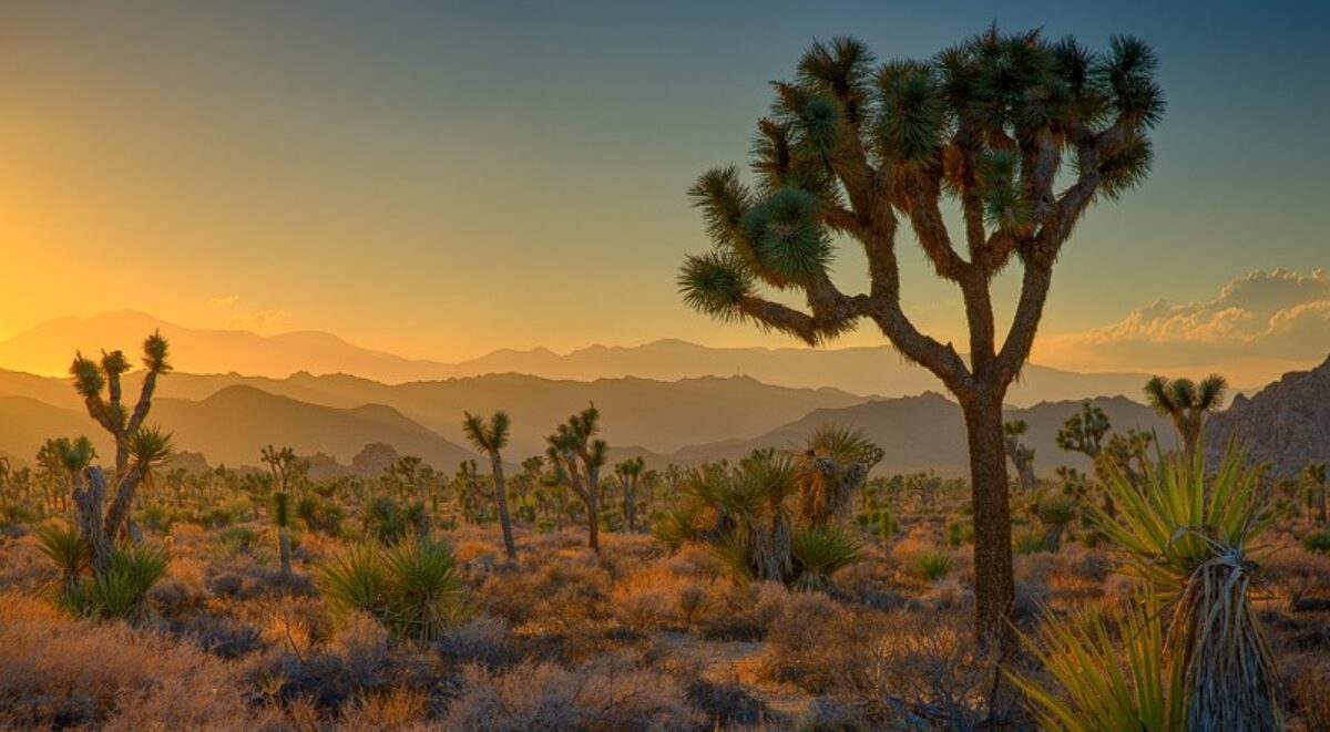
This photograph is a silhouette with a large dark foreground with the evening sky in the background. This histogram is a luminance histogram; that is, it ignores what little color there is in the image and just reports on shades of gray. (In many digital cameras RGB histograms are also available. They show each of the three color channels – red, green and blue – from the darkest shade of each color to its lightest. This can be very useful in many shooting situations that I’ll discuss later.)
The histogram above shows a spike toward the left of the graph and a second broader area in the middle. The spike on the left side, the shadow side, is the dark silhouette in the foreground. The broader area toward the center is the sky. That fact that this area is in the center tells us that the sky is neither dark nor light, something we can clearly see with our eyes. Tonalities that fall in the middle of the histogram like this are referred to as “mid-tones.” In the black and white world they would be called “neutral gray,’” a shade of gray that is perceived as being neither dark nor light. Understanding mid-tones is important to understanding how our camera’s light meter works but is not particularly relevant to this discussion.
Normal Exposure
In a normal exposure the histogram fits between the left and right sides. It doesn’t have to fill the entire range (we’ll talk more about this in a subsequent post) but it’s OK if it does. Here’s an example of just such a photograph. The subject is not particularly interesting and the light is horrible but the image illustrates the point. The histogram extends from the left side to the right.

Notice there is a little bit of space or breathing room between the left end of the histogram and the left side of the graph. The same is true for the right side. This is a well exposed image.
But not all images will have histograms that extend to both sides. Why? Because the dynamic range of the scene may not be as great as the dynamic range of the camera’s sensor. You see, what’s really going on here is the camera’s sensor has a maximum dynamic range that it is capable of capturing. The sensor’s dynamic range is the difference between the darkest and brightest parts of the scene that it can capture without loosing detail in the both the shadows and the highlights. The dynamic range is measured in f/stops and a typical digital camera may have a dynamic range of five or six f/stops.
So if you’re photographing a scene such as the one above where the dynamic range of the scene matches the dynamic range of the sensor, you get a histogram that nicely fits into the entire graph. But some of the scenes will have a dynamic range that is smaller than that of the camera’s sensor. And here’s what you get then. Again, the subject is blah, the light is horrible but the histogram illustrated the point.

This scene lacks the foreground shadows and the bright sky of the previous example. It’s dynamic range is dramatically reduced and the histogram reflects that. Also notice that the camera’s light meter centered the histogram, placing it in the mid-tone range.
These first two examples are ones of correctly exposed images. Next let’s take a look at what happens when an image is over- or underexposed.
Clipping
This next example shows the first image but now it is intentionally overexposed. You can see that clearly enough just from looking at it. It appears bright and washed out.

There are many areas in the image that have no detail whatsoever; these areas are pure white. The histogram reflects this situation; it is pushed up against the right (highlight) side – climbing the wall. This is highlight clipping. And since a large area of the image is overexposed, a proportionately large area of the histogram is crammed up against the right wall.
The opposite situation occurs when the image is underexposed.

The entire image appears dark and this is reflected in the histogram being well to the left of the mid-tone center. Areas of the image are pure black with no detail although the areas are not that large. That’s also reflected in the histogram which has shifted to the left (shadow) side. A small portion of the histogram has climbed the left wall but not as dramatically as the overexposed example. Still, there is some shadow clipping in this image.
Let’s look at the numbers. Digital cameras are computers and computers store all data as numbers. Images are captured by the sensor as points of light or pixels. So the luminance (lightness and darkness) of a pixel is stored as a number. Well, actually, it’s stored as three numbers – red, green and blue. When all three numbers are 0 you have pure black. The numbers at the left wall are (0,0,0). The numbers at the right wall depend on whether your images are captured at 8 or 16 bits per channel. Let’s go with 8 for this illustration. The smallest number that can be represented with 8-bit color is 0 (of course). The largest number is 255 (ask a computer geek to explain this if it doesn’t make sense to you). So if (0,0,0) is pure black and, in 8-bit color, (255,255,255) is pure white.
When you capture an image in your digital camera the intensity of the light at each pixel is translated into three numbers like (100,105,90) which happens to be the color of the leaves of a California live oak tree.
Clipping occurs when the pixels contain the extremes of these numbers. When a pixel’s values are (255,255,255) you have highlight clipping. When the values are (0,0,0) you have shadow clipping. It’s as simple as that.
The Worst Clipping
Both highlight clipping and shadow clipping are something to be avoided but are they equally ‘bad’ or is one worse than the other? This question has a very cut and dried answer. While we prefer avoiding both forms of clipping, highlight clipping is by far the worst. That’s because you can often recover at least some detail from shadow clipping. You may have some noise but that can often be handled with noise reduction plugins. But all too often there’s no recovering highlight clipping. There’s no detail, there’s no color, nothing. So, when I need to choose between highlight clipping and shadow clipping I’ll underexpose to preserve the highlights and accept whatever shadow clipping happens. This produces silhouettes which in many instances look really nice.
Clipping Is Not…
There are some misconceptions about clipping. One is that the histogram below shows clipping.

There are some that think that if a histogram peak touches the top like this one you have clipping. But that’s not the case at all. The large spike in the middle of the histogram is caused by the stucco wall that occupies a large area of the image. The RGB numbers for the stucco wall (in 8-bit color) are (130,130,122), nowhere near the clipping numbers of (0,0,0) or (255,255,255). The fact is these numbers are near the mid-tone numbers of (128,128,128). So the big spike in the middle of the graph just means that a large portion of the image is at or near the mid-tone. It’s NOT clipping.
At times during a photography workshop a student will point to a histogram with a huge spike like this one and ask if they have a clipping problem. Or they’ll ask what the best shape of a histogram is. I always respond with the question, “What’s happening on the right side of your histogram?” I want them to be aware of highlight clipping because I’ve lost more potentially exciting images due to highlight clipping than any other cause. The shape of the histogram doesn’t matter as long as it stays away from the right side. In fact, you have no control over the shape of the histogram. The only thing you have control over is where you place the histogram and that is controlled by the exposure. As we saw above, overexposure shifts the histogram to the right and underexposure shifts it to the left. You want to choose an exposure that avoids highlight clipping.
The shape of the histogram can affect the decisions you make regarding exposure and post processing and I’ll cover these in a later post. But for now, the most important rule in exposure, the first critical step in creating a compelling photograph is
AVOID HIGHLIGHT CLIPPING.
Join me on an upcoming workshop. Click here for more details.
To see more of my photographs click here.
(2709)